One Graph, Fifteen Spellings, a 28-Point Difference
Oracle wrote the same knowledge graph in 15 text formats and ran nine frontier model configurations over four benchmarks. Extraction barely notices, with 1.3 to 3.9 points of spread. Structural reasoning moves 28.4.
In one line. How a graph is spelled into a prompt is a measurable system parameter. It is worth 1.3 to 3.9 points on ontology extraction and 28.4 points on structural reasoning, and the three reasoning tiers of a single model family each prefer a different format, with the most accurate tier burning the fewest tokens.
1. Pricing the step nobody prices#
Take an ordinary pipeline. A user asks something that needs two hops, your retriever pulls the two-hop neighbourhood out of a graph database, caps it at 450 triples, and hands the result to a prompt.
How you spelled that neighbourhood out was probably an accident. A json.dumps call, a chunk of turtle copied from a tutorial, or a few sentences of “A knows B”. The paper says that accident is worth 28.2 percentage points on the same model and the same question.
The numbers come from Julien Yu, Mihaela Bornea, Avirup Sil and Katrin Kirchhoff at Oracle, in a paper accepted to EMNLP 2026 Findings. They ran 110 Wikidata questions through gpt-5.4 with the subgraph and the question held fixed, changing only the serialization. jsonld scored 41.8%. adjacency scored 13.6%.
The effect had been measured before. Talk like a Graph reported 4.8 to 61.8 points on synthetic graphs, and KG-LLM-Bench reported 17.5 points on knowledge-graph understanding. This paper widens the design space, puts reasoning effort into the panel, and adds an experiment on real retrieved subgraphs.
2. What the fifteen spellings are#
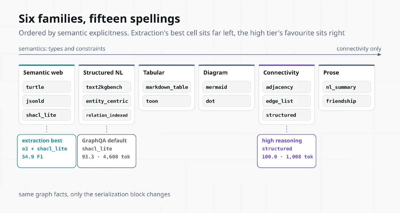
The authors group fifteen hand-written serializers into six families by how much semantic information they expose.
| Family | Formats | What it exposes |
|---|---|---|
| Semantic web and constraint views | turtle jsonld shacl_lite | Types, predicates, domain and range constraints |
| Structured natural language | text2kgbench entity_centric relation_indexed | Readable statements about entities and relations |
| Tabular | markdown_table toon | Node and edge tables |
| Diagram languages | mermaid dot | A drawing of the topology |
| Connectivity encodings | adjacency edge_list structured | The adjacency relation itself |
| Prose | nl_summary friendship | The graph narrated as sentences |
Two renders of the same five-node graph show the distance. structured writes it as two sets.
V = {0, 1, 2, 3, 4}
E = {(0,1), (0,2), (1,3), (2,3), (3,4)}
shacl_lite writes one shape per node, listing what that node connects to.
shape(3) {
  path adjacent -> node(1) ;
  path adjacent -> node(2) ;
  path adjacent -> node(4) ;
}
On GraphQA these two differ by more than a factor of four in input tokens.
The controls are tight. Inside one model-task instance every format shares the same instruction and the same graph facts, the random seed and node ordering stay put, and only the serialization block changes. Temperature is 0 everywhere except thinking-enabled claude-sonnet-4-6, which runs at the API default of 1.
3. Extraction hardly cares#
The first benchmark is ontology-driven extraction. The 2,014-sentence test split of Text2KGBench comes from 19 WebNLG domain ontologies, and the model has to pull every triple the ontology supports out of each sentence.
All nine configurations land between 45 and 55 F1. The per-format variation is 1.3 to 3.9 points. The best cell is o3 with shacl_lite at 54.9 F1, roughly 25 points above the 2023 baselines.
Discount that 25. The authors rescored offline with Hopcroft-Karp maximum matching where the original paper used a greedy matcher, and they say plainly that this delta is background context, outside the encoding effect. The part that belongs to serialization is the 1.3 to 3.9.
On cost, shacl_lite, text2kgbench and mermaid are efficient while scoring high, and turtle with jsonld cost substantially more tokens. All 19 ontologies are small, so context length never binds. What the cheaper formats save here is money.
The average hides one more thing. Split by domain, the head domains saturate (comicscharacter, university, scientist, astronaut) while the tail stays under 50 F1 (meanoftransportation, airport, monument, city). On unsaturated domains the cross-format spread reaches 6.1 points, above the 3.9 headline. Real workloads live in the tail.
4. Structural reasoning costs 28 points#
The second benchmark asks the model to compute graph properties from text. Degree, neighbours, components, shortest paths and triangle counts are the original tasks. On top of those sit seven harder operators.
Sensitivity rises with difficulty and falls with reasoning effort.
| Benchmark | Scale | Cross-format spread |
|---|---|---|
| GraphQA, gpt-5.4 default | 11 tasks, n from 8 to 50 | 4.8 pp |
| GraphQA, grok-4-fast non-reasoning | same | 17.0 pp |
| GraphQA-Hardened | n from 35 to 75, 7 extra operators | 4.2 to 28.4 pp |
| GraphQA-Topology | n fixed at 50, 6 generators | 5.5 to 16.7 pp |
| Wikidata subgraphs | 10 seeds, 110 questions | 24.5 to 28.2 pp |
None of the seven added operators can be read off a local edge list. They ask for k-core size, graph diameter, maximum clique, the second-shortest simple path, the top betweenness node, the local clustering coefficient, and the count of neighbours above a degree threshold.
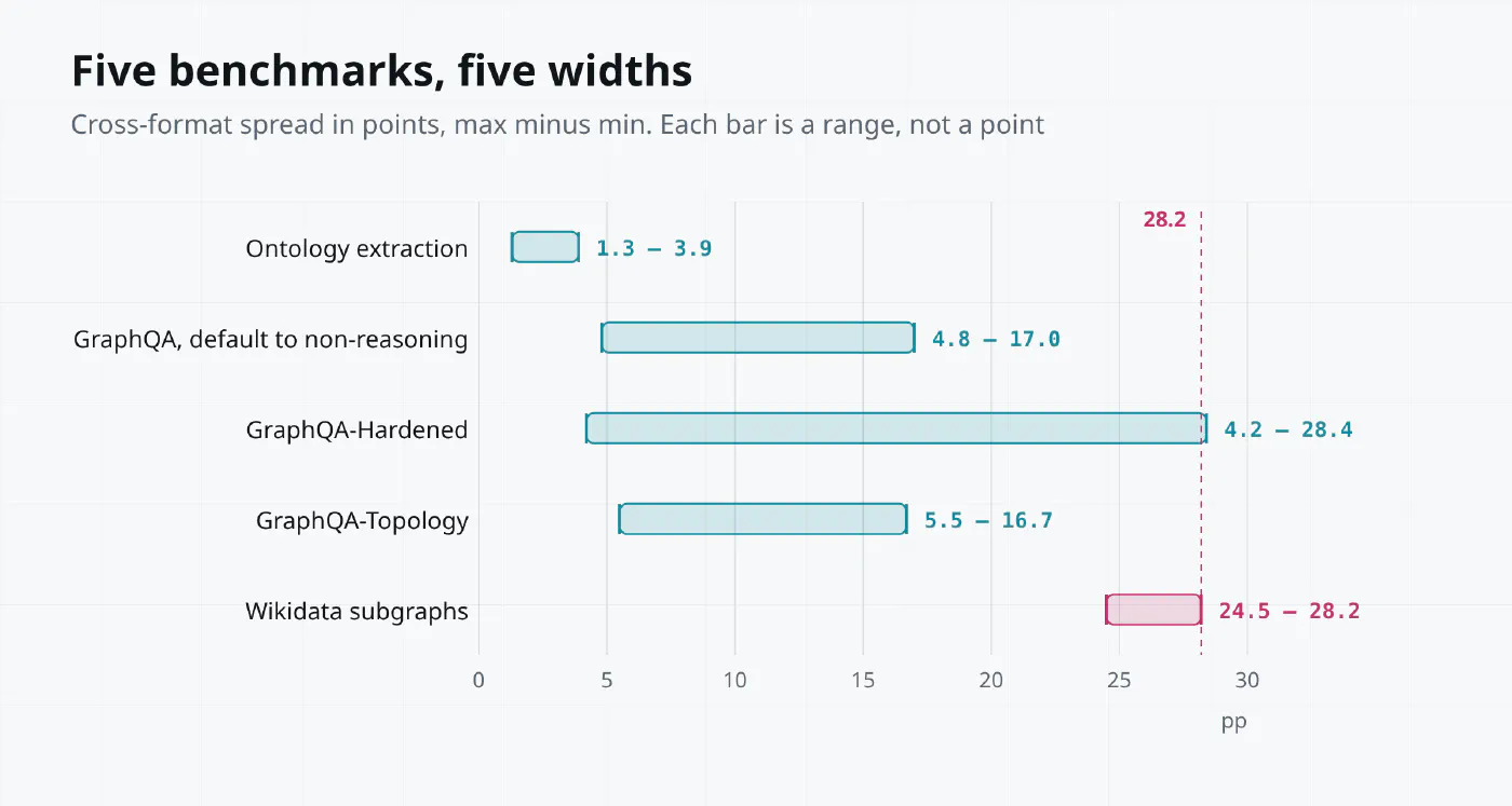
The interval length is the number that matters. Swap formats on extraction and you gain almost nothing. Swap formats on structural reasoning and you can lose a third of your score.
5. Three tiers, three favourite formats#
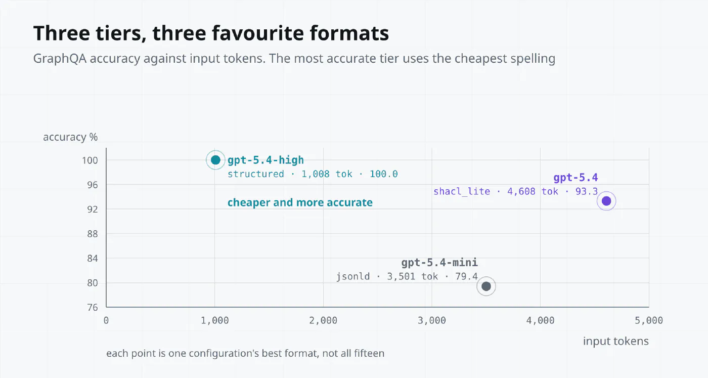
One model family produces three different favourite formats.
| Configuration | Best format | GraphQA accuracy | Input tokens |
|---|---|---|---|
| gpt-5.4-mini | jsonld | 79.4 | 3,501 |
| gpt-5.4 default | shacl_lite | 93.3 | 4,608 |
| gpt-5.4 high reasoning | structured | 100.0 | 1,008 |
The tier that saturates accuracy does it with the cheapest format, 4.5 times cheaper than the default tier’s favourite. The default tier needs the four thousand tokens of shape constraints that shacl_lite provides. The high tier reads two sets and is done.
Preferences flip between tiers of the same family, so one global best format does not exist. A pipeline running a cheap model on the long tail and an expensive one on hard cases cannot pick one spelling and be fair to both.
6. Pure connectivity collapses on real graphs#
Synthetic questions ask for topological quantities. Real knowledge-graph questions often ask for the predicate and the type themselves. “How many films have at least one director” is a question about the director edge, and a format that drops edge labels drops the answer.
The real-graph experiment uses 10 seed entities across films, scientists, cities and companies, retrieves the two-hop neighbourhood of each, and caps the context at 450 triples. Entity labels become consistent anonymous identifiers while predicate labels stay. The 110 questions split into 31 relation-specific aggregations, 31 type aggregations, and 48 reachability questions. Gold answers are computed on the canonical subgraph before serialization, so all fifteen formats carry the same facts.
Pseudonymizing the entities is the load-bearing design choice. It removes the option of answering from memory about a famous scientist and leaves only the text.
Both models rank jsonld first and turtle second.
| Model | Best | Worst | Spread |
|---|---|---|---|
| gpt-5.4 | jsonld 41.8% | adjacency 13.6% | 28.2 pp |
| gpt-5.4-mini | jsonld 30.9% | nl_summary 6.4% | 24.5 pp |
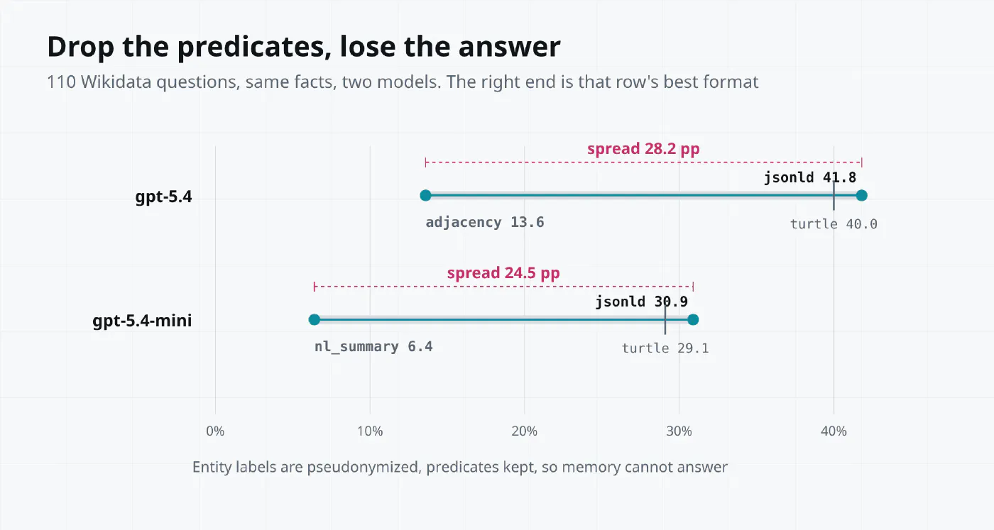
adjacency is cheap and effective on synthetic graphs and lands at 13.6% here. It throws away the predicates and the types, which is exactly what the questions ask about.
The authors add a limit of their own. The family labels are descriptive, not a causal decomposition, and no single characteristic explains the rankings. The same organisation of information can perform well on one task and badly on another.
7. Letting the model pick per question#
If the best format varies per question, pick per question. The authors build a selector with five candidate formats and five parallel scoring calls, and hand the highest-scoring rendering to a single answer call. A scoring call sees the question, the candidate’s name, that format’s calibration accuracy, and the graph rendered in it. Selector rationales never reach the answer model.
Calibration and test are 105 questions each, drawn from the same generator with disjoint seed families. Calibration is an offline audit of 7 tasks by 15 formats, 1,575 calls, which produces a per-task accuracy prior table.
| Policy | Accuracy | API cost | Latency |
|---|---|---|---|
| Global fixed best | 66.67% | 1.00x | one call |
| Task-level router | 64.76% | near 1.00x | one call |
| Five-way majority vote | 71.43% | 5.69x | 9.1 s |
| Per-question selector | 76.19% | 3.71x | 9.4 s |
| Post-hoc oracle on the same slate | 82.86% | n/a | n/a |
The selector beats fixed-best by 9.52 points, with a paired bootstrap 95% interval of [+1.90, +16.19] and a McNemar test at p=0.013. Task-level routing scores 64.76, below fixed-best, so the gain comes from per-question judgement and task priors alone do not explain it.
3.71 times the money for 9.52 points looks expensive on first read. Majority voting spends 5.69 times and reaches 71.43, so the selector buys more per dollar. It also captures about 59% of the slate-restricted headroom, leaving the rest to a better scorer.
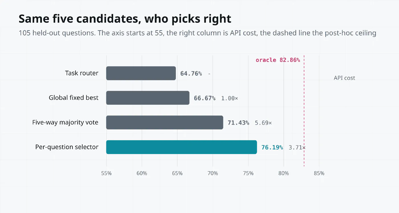
The result holds inside one distribution. Test questions come from independently seeded GraphQA-Hardened graphs, and gpt-5.4 serves as both selector and generator. Transfer across datasets, graph distributions and model pairings is left as future work.
8. The check you can run yourself#
Before adopting any of this, find out whether your task sits in the narrow band or the wide one. The check takes an afternoon.
- Fix 20 to 50 questions and one graph. If the retriever returns a different subgraph each run, the comparison means nothing.
- Pick three to five formats spanning the spectrum.
jsonld,shacl_lite,structured,adjacencyandnl_summarycover it. - Temperature 0, response cache off, three rounds per format.
- Log two columns per question, correct or not, and input tokens.
- Compute two numbers, the cross-format spread (max minus min) and the standard deviation across the three rounds of one format.
The decision rule is short enough to copy.
# spread_check.py, a script for this post, not repository code
def verdict(spread_pp: float, run_std_pp: float) -> str:
    if spread_pp < 3:
        return "fix one format and stop spending time here"
    if spread_pp < 10:
        return "fix one format per task group, skip the selector"
    if run_std_pp * 3 > spread_pp:
        return "the gap is not stable, add samples and rerun"
    return "the gap is real, a per-question selector is worth building"
The last branch leans on a control in the paper. Three independent decodes of all fifteen formats, 20,250 calls, gave a per-format run-to-run standard deviation of 1.5 points, against a between-format spread 7.7 times larger on average. If your repeat noise approaches the gap, you measured noise.
9. Two questions still open#
The first is transfer. The selector and the generator are the same model, and the pipeline has only run on GraphQA-Hardened. Whether the same scoring prompt works with Claude or an open-weight model is untested, and the scoring judgement itself depends on model capability.
The second is the tail. Extraction averages 45 to 55 F1 across domains, the tail sits under 50, and cross-format spread there reaches 6.1 points. Most production workloads live in the tail, which is the thinnest part of this study.
There is one more limit the authors name themselves. Every model in the panel is a closed commercial system, so prior exposure to particular formats cannot be ruled out. Open-weight models let you rerun the panel and test whether that exposure mattered.
References#
- Graph Serializations for Reasoning LLMs , EMNLP 2026 Findings
- Talk like a Graph , the source of GraphQA
- KG-LLM-Bench , the 17.5-point result
- Text2KGBench , ontology-driven extraction benchmark
- SHACL
, where
shacl_litecomes from - JSON-LD 1.1
, the
jsonldspecification